8 UI Applications
We have developed a few UI applications for exploring LT-GEE time series data. They can be found in our public GEE repository. To access the applications, visit this URL: https://code.earthengine.google.com/?accept_repo=users/emaprlab/public). It will add the users/emaprlab/public repository to your GEE account. Once added, the repository can be found within the Reader permission group of your GEE scripts library. There you’ll find the following user interface applications that run as GEE Apps (i.e. do not require you load and run a script).
- [UI LandTrendr Download MultiTool] | link |
- UI LandTrendr Pixel Time Series Plotter | link | source and LandTrendr-fitted data for a pixel
- UI LandTrendr Change Mapper | link | map disturbances and view attributes
- UI LandTrendr Fitted Index Delta RGB Mapper | link | visualize change and relative band/index information
- UI LandTrendr Time Series Animator | link | make an animated GIF from a LandTrendr FTV annual time series
Additionally, we have developed a script-based UI tool that combines many of the aforementioned functions, plus adds functionality to some of the components. + [LandTrendr Data Visualization and Download Tool] | link
*Note: The link above is static. To access the most up-to-date version of the script, from your GEE interface open the script **users/emaprlab/public:LT-data-download/LT-Data-Visualization-Download-App_v1.0*
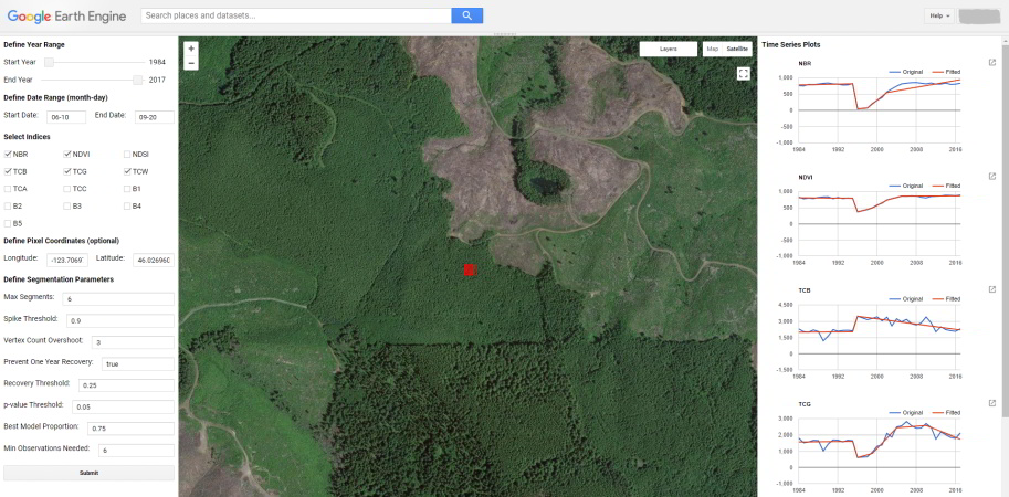
8.1 UI LandTrendr Pixel Time Series Plotter
The UI LandTrendr Pixel Time Series Plotter will plot the Landsat surface reflectance source and LandTrendr-fitted index for a selected location. The script is useful for simply exploring and visualizing the spectral-temporal space of a pixel, for comparing the effectiveness of a series of indices for identifying landscape change, and for parameterizing LandTrendr to work best for your study region.
8.1.1 Steps
- Click on the script to load it and then click the Run button to initialize the application.
- Drag the map panel to the top of the page for better viewing.
- Define a year range over which to generate annual surface reflectance composites.
- Define the date range over which to generate annual composites. The format is (month-day) with two digits for both month and day. Note that if your study area is in the southern hemisphere and you want to include dates that cross the year boundary to capture the summer season, this is not possible yet - it is on our list!
- Select spectral indices and bands to view. You can select or or many.
- Optionally define a pixel coordinate set to view the time series of, alternatively you’ll simply click on the map. Note that the coordinates are in units of latitude and longitude formatted as decimal degrees (WGS 84 EPSG:4326). Also note that when you click a point on the map, the coordinates of the point will populate these entry boxes.
- Define the LandTrendr segmentation parameters. See the LT Parameters section for definitions.
- Either click a location on the map or hit the Submit button. If you want to change anything about the run, but keep the coordinate that you clicked on, just make the changes and then hit the Submit button - the coordinates for the clicked location are saved to the pixel coordinates input boxes.
Wait a minute or two and plots of source and LandTrendr-fitted time series data will appear for all the indices you selected. The next time you click a point or submit the inputs, any current plots will be cleared and the new set will be displayed.
8.1.2 Under the hood
- Landsat 8 is transformed to the properties of Landsat 7 using slopes and intercepts from reduced major axis regressions reported in Roy et al 2016 Table 2
- Masking out clouds, cloud shadows, and snow using CFMASK product from USGS
- Medoid annual compositing
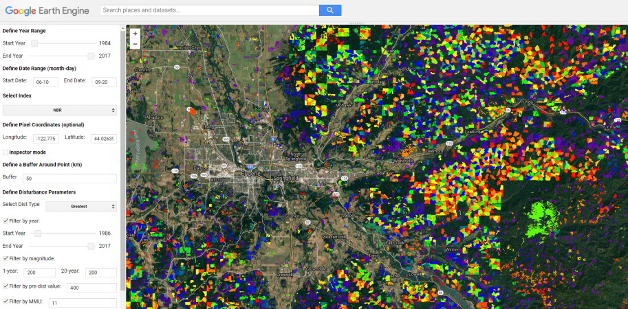
8.2 UI LandTrendr Change Mapper
The UI LandTrendr Change Mapper will display map layers of change (vegetation loss or gain) attributes including: year of change detection, magnitude of change, duration of change event, and pre-change spectral value.
8.2.1 Steps
- Define a year range over which to build a Landsat time series to identify change - best to set this close to the maximum range, you can filter changes by year in a different setting below.
- Define the date range over which to generate annual Landsat image composites. The format is (month-day) with two digits for both month and day. Note that you can cross the year boundary, which is desirable if your study area is in the southern hemisphere, for example, Start Date: 11-15 and End Date: 03-15. If the start day month is greater than the end day month, then the function will composite across the new year, and assign the year of the composite as the new year.
- Select spectral index or band to use for change detection.
- Select the features you would like to mask from the imagery - these features are identified from the CFMASK quality band included with each image.
- Optionally provide a pixel coordinate set to define the center of the change map, alternatively you will simply click on the map location desired. Note that the coordinates are in units of longitude and latitude formatted as decimal degrees (WGS 84 EPSG:4326). Also note that when you click a point on the map, the coordinates of the point will populate these entry boxes. If you choose to enter coordinates, then you must click the submit button at the bottom of the control panel once all options are selected to generate the map.
- Define a buffer around the center point defined by a map click or provided in the longitude and latitude coordinate boxes from step 5. The units are in kilometers. It will draw and clip the map to the bounds of the square region created by the buffer around the point of interest.
- Define the vegetation change type you are interested in - either vegetation gain or loss.
- Define the vegetation change sort - should the change be the greatest, least, longest, etc. This applies only if there are multiple vegetation changes of a given type in a pixel time series. It is a relative qualifier for a pixel time series.
- Optionally filter changes by the year of detection. Adjust the sliders to constrain the results to a given range of years. The filter is only applied if the Filter by Year box is checked.
- Optionally filter changes by magnitude. Enter a threshold value and select a conditional operator. For example, if you selected the change type as vegetation loss defined by NBR and wanted only high magnitude losses shown, you would maybe want to keep only those pixels that had greater than 0.4 NBR units loss - you would set value as 400 (NBR scaled by 1000 - keep reading for more on this) and select the > operator. The value should always be positive which is on a scale of either vegetation loss or gain with 0 being no loss or gain and high values being high loss or gain, where gain and loss are defined by the vegetation change type selected above. Values should be multiplied by 1000 for ratio and normalized difference spectral indices (we multiply all the decimal-based data by 1000 so that we can convert the data type to signed 16-bit and retain some precision), and keep in mind that surface reflectance bands are multiplied by 10000 according to LEDAPS and LaSRC processing The filter is only applied if the Filter by Magnitude box is checked.
- Optionally filter by change event duration. Enter a threshold value and select a conditional operator. For example, if you only want to display change events that occurred rapidly, you would maybe set the value as 2 (years) and the operator as < to retain only those changes that completed within a single year. The filter is only applied if the Filter by Duration box is checked.
- Optionally filter by pre-change spectral value. This filter will limit the resulting changes by those that have a spectral value prior to the change either greater or less than the value provided. Values should be multiplied by 1000 for ratio and normalized difference spectral indices (we multiply all the decimal-based data by 1000 so that we can convert the data type to signed 16-bit and retain some precision), and keep in mind that surface reflectance bands are multiplied by 10000 according to LEDAPS and LaSRC processing. The filter is only applied if the Filter by Pre-Dist Value box is checked.
- Optionally filter by a minimum disturbance patch size, as defined by 8-neighbor connectivity of pixels having the same year of change detection. The value is the minimum number of pixel in a patch. The filter is only applied if the Filter by MMU box is checked.
- Define the LandTrendr segmentation parameters. See the LT Parameters section for definitions.
- Optionally submit the options for processing. If you have provided longitude and latitude coordinates to define the map center in step 5, you must submit the task. If you have generated a map and want to change a parameter, do so and then redraw the map by pressing this submit button.
Inspector mode selector. In the right hand panel the app there is a check box for whether to interact with the map in Inspector mode or not. When inspector mode is activated, map clicks will retrieve change event attributes for the clicked pixel and display them in the right hand panel. When deactivated, a map click will start mapping changes for the region surrounding the clicked point.
8.2.2 Under the hood
- Landsat 8 is transformed to the properties of Landsat 7 using slopes and intercepts from reduced major axis regressions reported in Roy et al 2016 Table 2
- Masking out clouds, cloud shadows, and snow using CFMASK product from USGS
- Medoid annual compositing
8.2.3 ToDo
- Option to export the map layers
- Allow input of a user drawn area or import of a feature asset or fusion table
- auto stretch to different indices - right now it is defaulting stretch for NBR
- Force absolute value for magnitude filter inputs
- Handle input of unscaled decimal values for the pre-dist and magnitude filter parameters
8.3 UI LandTrendr Fitted Index Delta RGB Mapper
The UI LandTrendr Fitted Index Delta RGB Mapper will display an RGB color map representing spectral band or index values at three time slices. Formally, it is referred to as write function memory insertion change detection. Each color red, green, and blue are assigned a year of spectral data, then those data are composited to an RGB image where each of red, green, and blue are mixed by weighting of the spectral intensity for the year represented by each color. It is useful as a quick way to visualize change or non-change over time along with providing a relative sense for spectral intensity. If I’m just exploring change in an area, I’ll often use this before strictly mapping disturbance, because I get a sense for spectral distribution and spatial pattern. Once you get a handle on interpreting the colors it is really quite an interesting and useful visualization.
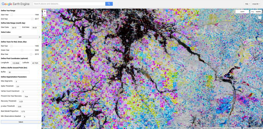
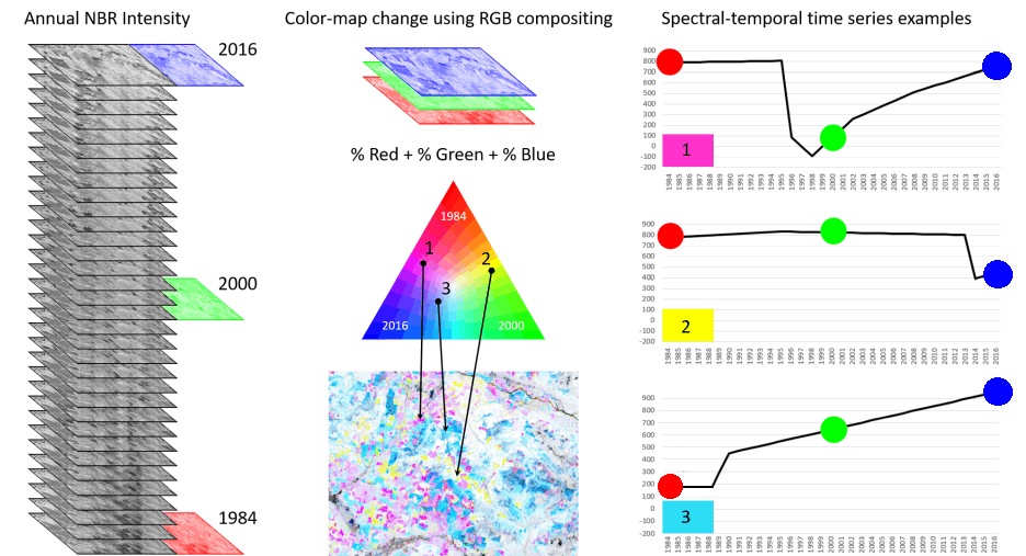
The following figure is a guide to help interpret the colors.
8.3.1 Steps
- Click on the script to load it and then click the Run button to initialize the application.
- Drag the map panel to the top of the page for better viewing.
- Define a year range over which to identify disturbances - best to set this close to the maximum range, you can filter disturbances by year in a different setting below.
- Define the date range over which to generate annual composites. The format is (month-day) with two digits for both month and day Note that if your study area is in the southern hemisphere and you want to include dates that cross the year boundary to capture the summer season, this is not possible yet - it is on our list!
- Select spectral index or band to use for segmentation and change detection.
- Define years to represent red, green, and blue color in the final RGB composite.
- Optionally define a pixel coordinate set to define the center of the disturbance map, alternatively you’ll simply click on the map. Note that the coordinates are in units of latitude and longitude formatted as decimal degrees (WGS 84 EPSG:4326). Also note that when you click a point on the map, the coordinates of the point will populate these entry boxes.
- Define a buffer around the center point defined by a map click or provided in the latitude and longitude coordinate boxes from step 6. The units are in kilometers. It will draw and clip the map to the bounds of the square region created by the buffer around the point of interest.
- Define the LandTrendr segmentation parameters. See the LT Parameters section for definitions.
- Either click on the map or hit the Submit button to draw the map - wait a few minutes for the process to complete.
8.3.2 Under the hood
- Landsat 8 is transformed to the properties of Landsat 7 using slopes and intercepts from reduced major axis regressions reported in Roy et al 2016 Table 2
- Masking out clouds, cloud shadows, and snow using CFMASK product from USGS
- Medoid annual compositing
- 2 standard deviation stretch on the selected band or spectral index
8.3.3 ToDo
8.4 UI LandTrendr Time Series Animator
The UI LandTrendr Time Series Animator will make an animated GIF from a Landsat time series that has been smoothed by LandTrendr spectral-temporal segmentation.
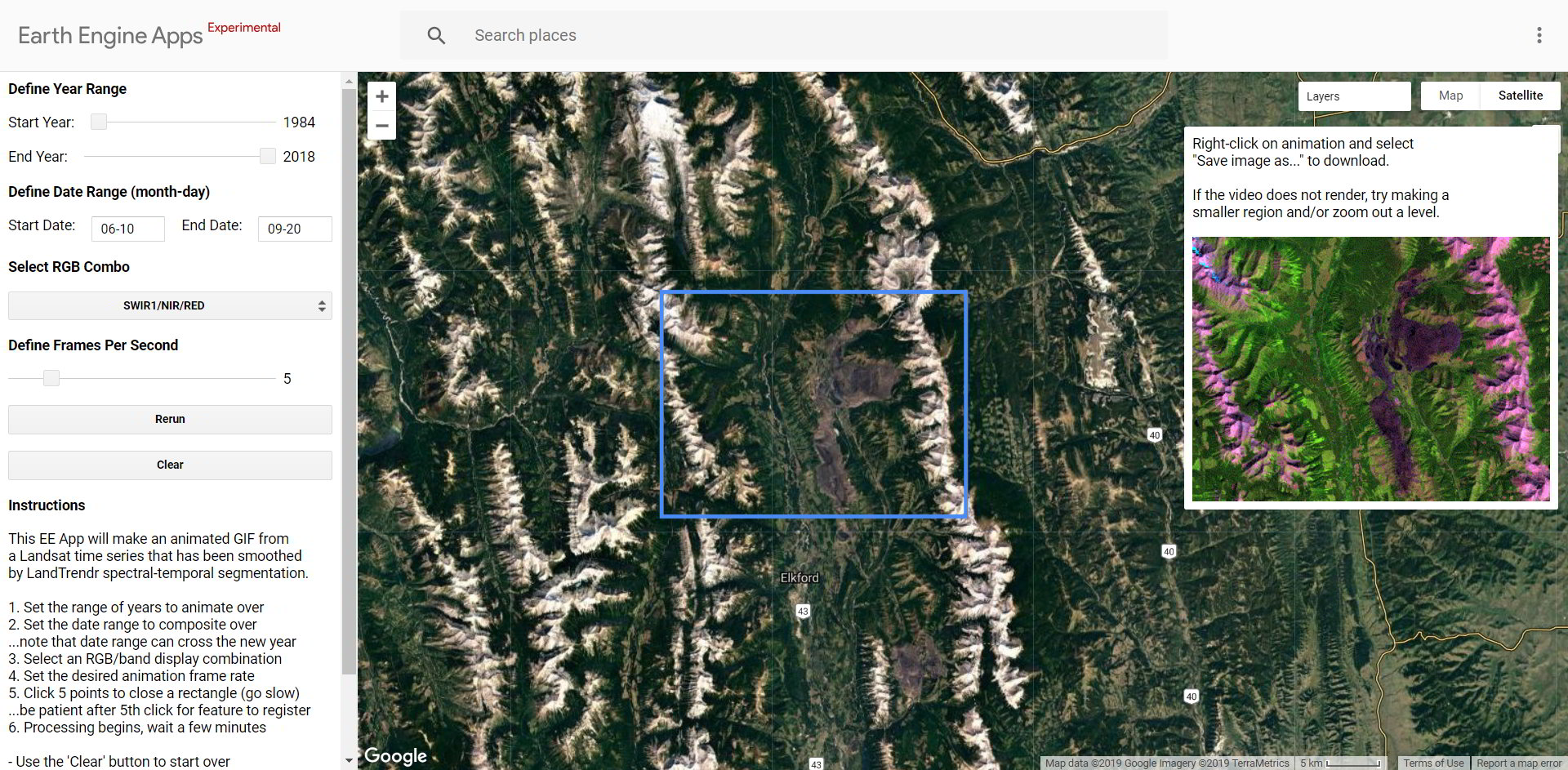
8.4.1 Steps
- Set the range of years to animate over,
- Set the date range to composite over. Note that date range can cross the new year.
- Select an RGB/band display combination.
- Set the desired animation frame rate.
- Click 5 points to close a rectangle (go slow). Be patient after 5th click for feature to register.
- Processing begins, wait a few minutes.
- Use the ‘Clear’ button to start over.
- Change RGB combo and ‘Rerun’ on same region.
- If a video does not render, try making a smaller region and/or zoom out a level.
8.4.2 Credit
This application uses a modified version of a drawing tool originally developed by Gennadii Donchyts.
8.5 UI LandTrendr Visualilzation and Download Tool
- [LandTrendr Data Visualization and Download Tool] | link
*Note: The link above is static. To access the most up-to-date version of the script, from your GEE interface open the script **users/emaprlab/public:LT-data-download/LT-Data-Visualization-Download-App_v1.0*
8.5.1 Steps
- In your own GEE session, navigate to the “Reader” section of your scripts and open the file “users/emaprlab/public:LT-data-download/LT-Data-Visualization-Download-App_v1.0”
- Run the app (click the “Run” button)
- There are components to this UI for pixel time-series, RGB image generation, and change mapping. Expand the section you want, set parameters using steps similar to those listed above, and submit them.
- If you generate a map or image, you can subsequently switch back to the pixel-mode and query the time-series of individual pixels. This is useful for evaluating if you’ve chosen parameters for the mapping well.
- You can also download outputs from the maps, and point to your own vector-based assets to constrain analysis.