5 LT-GEE Outputs

The results of LT-GEE include (Fig 5.1):

The year of observations per pixel time series; x-axis values in 2-D spectral-temporal space; (default)
The source value of observations per pixel time series; y-axis values in 2-D spectral-temporal space; (default)
The source value of observations fitted to segment lines between vertices (FTV) per pixel time series; y-axis values in 2-D spectral-temporal space; (default)
The root mean square error (RMSE) of the FTV values, relative to the source values; (default)
Complete time series FTV values for additional bands in the collection greater than band 1; y-axis values in 2-D spectral-temporal space; (optional)

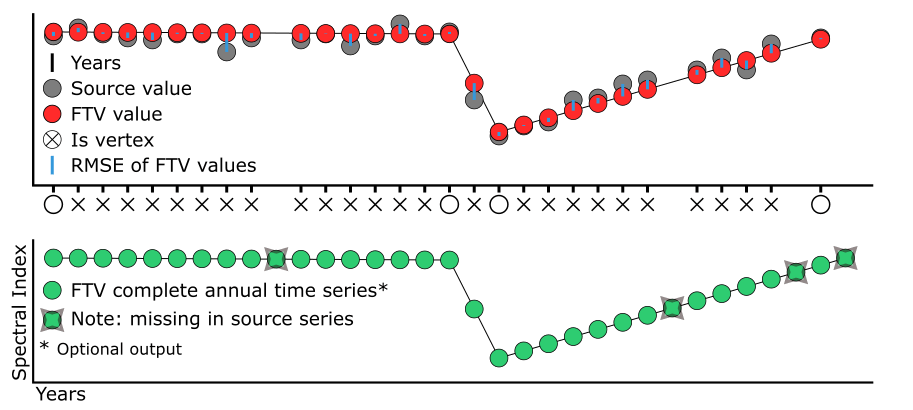
Fig 5.1. A visual diagram of what data are returned from LT-GEE. Every legend item is returned as an output.

The results of LT-GEE are not immediately ready for analysis, display, or export as maps of change or fitted time series data. Think of each pixel as a bundle of data that needs to be unpacked. The packaging of the data per pixel is similar to a nested list in Python or R. The primary list looks something like this:

[[Annual Segmentation Info], Fitting RMSE, [Fitted Time Series n]]

In the GEE construct, this primary list is an image with at least 2 bands, one that contains annual segmentation information and one that contains the RMSE of the segmentation fit. Additionally, if the input image collection to LT-GEE contained more than one band, then each band following the first will be represented as a spectrally fitted annual series (Fig 5.2 and Fig 5.3).

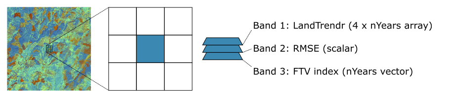
Fig 5.2. The results of LT-GEE are essentially a list of lists per pixel that describe segmentation and optionally provide fitted annual spectral data (FTV). The output is delivered as a GEE image with at least 2 bands, one that contains annual segmentation information and one that contains the RMSE of the segmentation fit. Additionally, if the input image collection to LT-GEE contained more than one band, then each band following the first will be represented as a spectrally fitted annual series (FTV).

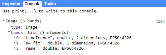
Fig 5.3. The results of LT-GEE printed to the GEE console. The ‘LandTrendr’ and ‘rmse’ are included by default, ‘B4_fit’ is included because Landsat TM/+ETM band 4 (B4) was included as the second band in the input collection.

5.1 LandTrendr Band

The ‘LandTrendr’ band is a 4 x nYears dimension array. You can subset it like this:

var LTresult = ee.Algorithms.TemporalSegmentation.LandTrendr(run_params); // run LT-GEE
var segmentationInfo = LTresult.select(['LandTrendr']); // subset the LandTrendr segmentation info

It contains 4 rows and as many columns as there are annual observations for a given pixel through the time series. The 2-D ‘LandTrendr’ annual segmentation array looks like this:

[
  [1985, 1986, 1987, 1988, 1989, 1990, 1991, 1992, 1993, 1994, 1995, 1996, 1997, ...] // Year list 
  [ 811,  809,  821,  813,  836,  834,  833,  818,  826,  820,  765,  827,  775, ...] // Source list
  [ 827,  825,  823,  821,  819,  817,  814,  812,  810,  808,  806,  804,  802, ...] // Fitted list
  [   1,    0,    0,    0,    0,    0,    0,    0,    0,    0,    0,    0,    1, ...] // Is Vertex list
]

Row 1 is the observation year.
Row 2 is the observation value corresponding to the year in row 1, it is equal to the first band in the input collection.
Row 3 is the observation value corresponding to the year in row 1, fitted to line segments defined by breakpoint vertices identified in segmentation.
Row 4 is a Boolean value indicating whether an observation was identified as a vertex.

You can extract a row using the GEE arraySlice function. Here is an example of extracting the year and fitted value rows as separate lists:

var LTresult = ee.Algorithms.TemporalSegmentation.LandTrendr(run_params); // run LT-GEE
var LTarray = LTresult.select(['LandTrendr']); // subset the LandTrendr segmentation info
var year = LTarray.arraySlice(0, 0, 1); // slice out the year row
var fitted = LTarray.arraySlice(0, 2, 3); // slice out the fitted values row

The GEE arraySlice function takes the dimension you want to subset and the start and end points along the dimension to extract as inputs.

5.2 RMSE

The ‘rmse’ band is a scalar value that is the root mean square error between the original values and the segmentation-fitted values.

It can be subset like this:

var LTresult = ee.Algorithms.TemporalSegmentation.LandTrendr(run_params); // run LT-GEE
var segmentationInfo = LTresult.select(['rmse']); // subset the rmse band

5.3 FTV

If the the input image collection included more than one band, the proceeding bands will be included in the output image as FTV or fit-to-vertice data bands. The segmentation, defined by year of observation, of the first band in the image collection is imparted on these bands. If there were missing years in the input image collection, they will be interpolated in the FTV bands. If years at the beginning or end of the series are present, the value will be set as the first/last known value.

It can be subset from the primary output image by selection of the band name, which will be the the concatenation of the band name from the input image collection and ’_fit’, as in ‘B4_fit’. Here is an example of subsetting an FTV ‘fit’ band:

var LTresult = ee.Algorithms.TemporalSegmentation.LandTrendr(run_params); // run LT-GEE
var B4ftv = LTresult.select(['B4_fit']); // subset the B4_fit band

If you’re unsure of the band names, you can view the band names by printing the results to the GEE console.

var LTresult = ee.Algorithms.TemporalSegmentation.LandTrendr(run_params); // run LT-GEE
print(LTresult)

Then expand in the ‘Image’ and ‘Band’ objects in the console.